How to quickly use the Excel VLOOKUP function

What is the VLOOKUP function

Microsoft Excels VLOOKUP function is a search or query function that is able to find information in a table by using a lookup value that can be associated with other values on the same row. This is often referred to as a ‘key’ value. Is is similar to a SQL find function where a key value will be used to extract other information stored in the same record or row.

Why would I use the VLOOKUP function

Suppose you manage store inventory and you have the SKU value for your product but you would like to know the name or price of the SKU you have. Using the VLOOKUP function, you can input your known value, in this case SKU, and the function will return any associated information found in the same row as the SKU.

Other uses for VLOOKUP could be finding a students name by their student ID number or finding a birthday by using a name. The only requirement is the data must be structured vertically and the associated value needs to be stored to the right and in the same row as the lookup or key value.

How do I use the VLOOKUP function

• The user must have a lookup value associated with other information in a table.
• The table must be vertical with all data organized by row.
• The result value column distance from the lookup value must be determined.
• A location for the output of the lookup must me known.

How do I type the VLOOKUP function into Excel

The formula syntax for VLOOKUP is:

=VLOOKUP (lookup_value, table_array, column_index_num, [range_lookup])

What values will the VLOOKUP function require

lookup_value – The value that will be look up or searched for.

table_array – The vertical table area where related data is organized by row.

column_index_num – How many column away is the related value of interest.

[range_lookup] – True: Approximate match to the lookup value, False: Exact match to the lookup value.

Is there anything else I need to know about the VLOOKUP function

VLOOKUP only looks to the right of the look up column. It is recommended that the look up column be the very left column so the function can access all other related cells.

Always use absolute references with the table_array and possibly the lookup_value. This will permit fill-down of formulas that reference back to the original table selection.

Store values with the correct type. If you are using a date, make sure it is formatted as a date. This is particularly relevant to the first column of cells in the table_array. This will prevent matching errors, especially when using approximate matching. Avoid matching on text values when possible.

Always sort the first column of the table_array when using the approximate match (range_lookup = True). This is because VLOOKUP will match the first cell that is approximately the lookup_value.

Wildcard characters can be used when using the exact match option (range_lookup=False). The wildcards are * for multiple characters and ? matches a single character. To escape the matching function of the * and ?, escape the search character with a ~. Do this when you want to search for the actual * and ? characters.

If your first column uses text as the matching characters, make sure there are no erroneous characters or whitespace. Common erroneous characters are straight quotes ( ` ) or other non-printing characters. Use the TRIM or CLEAN functions to fix whitespace problems.

Example use of the VLOOKUP function

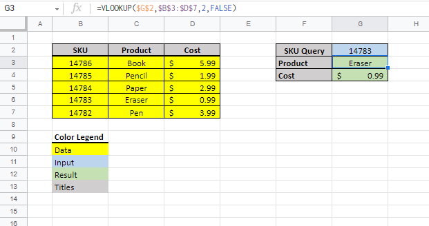
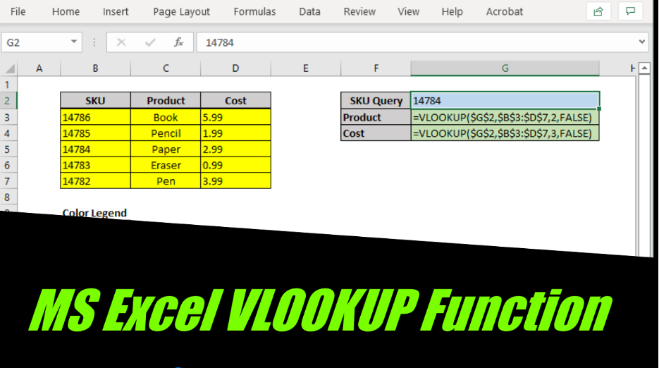
In this example, there is a table of products with the product name and price of each SKU. VLOOKUP will be used to look up the product name and price by the SKU value. Note the color legend, the only value input is the SKU Query, the results are the product and cost.

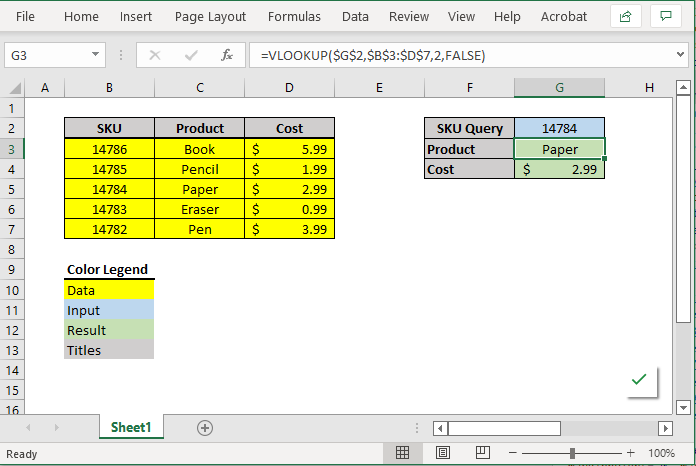
In the above example, the SKU Query value is set at 14784. VLOOKUP is used to retrieve the product name of “Paper” and price of $2.99.

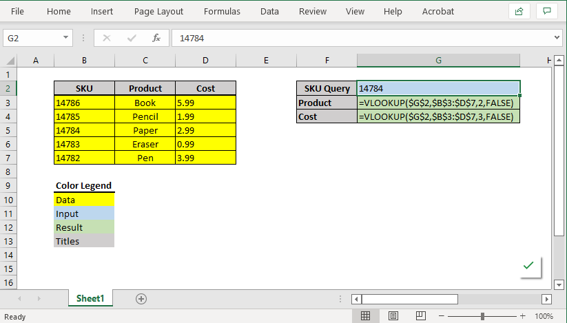
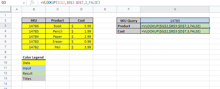
Exploring the formulas in use it can be seen that the VLOOKUP formula is used in the Product and Cost result cells.

=VLOOKUP($G$2,$B$3:$D$7,2,FALSE)

=VLOOKUP($G$2,$B$3:$D$7,3,FALSE)

The range_lookup value in this example is set to FALSE to find the exact match. The SKU values are very similar in number sequence. As has been said, if using the approximate range_lookup function, erroneous results may result.

To increase the reliability of the VLOOKUP function, it can be combined with the IFNA function to return a message indicating the lookup value does not return anything. By default, the function returns NA if no match is found.

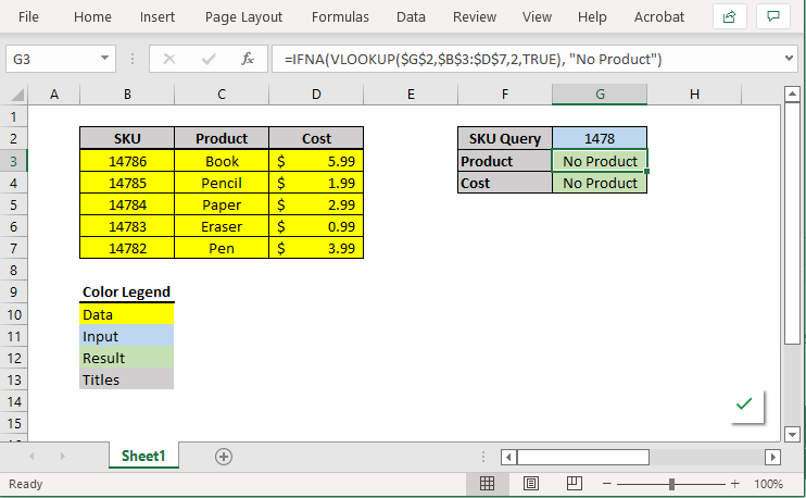
We used the lookup value of 1478 which is not in the first column of our table (SKU). Using the IFNA function, the spreadsheet alerts that there is no match by filling the cells with the text “No Product”.

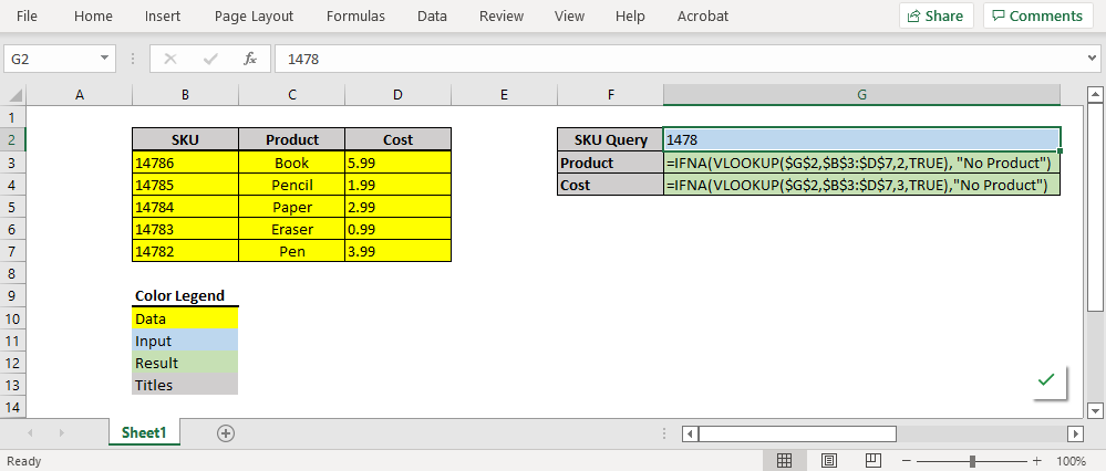
The formulas used to produce the “No Product” outcomes in the Product and Cost cell are.

How do I use the Excel VLOOKUP function in Google Sheets

Use of the Excel VLOOKUP function is exactly the same in Google Sheets. The syntax, inputs, outputs, and optional exact match are the same between both software packages. The screen shots from Google Sheets provide an example of what to expect when using VLOOKUP function in Google Sheets.